
Unleash the Secrets: The Ultimate Guide to Choosing the Perfect Black Dog Raincoat!
When it comes to our furry friends, ensuring their comfort and well-being is a top priority, especially during inclement weather. Keeping dogs dry during rainy seasons is not just about avoiding muddy paws; it’s essential for their health. For black dogs, a well-fitted raincoat not only provides functional benefits but also enhances their visibility against dark, rainy backgrounds. As we explore the various options and features available in black dog raincoats, we’ll also touch on different factors to consider to help you make an informed choice for your canine companion.
Understanding the Need for a Black Dog Raincoat
Rainy weather can pose various challenges for dogs, making raincoats a vital accessory. Firstly, keeping a dog dry is critical to prevent health issues such as hypothermia or skin infections that can occur when they are damp for extended periods. A raincoat offers protection from chilling winds and heavy downpours, ensuring your pet remains comfortable and warm. Additionally, raincoats can help minimize the mess that comes with wet fur, making post-walk clean-ups much easier. Beyond health benefits, a raincoat can transform a dreary walk into an enjoyable experience, allowing you and your furry friend to embrace the outdoors together, regardless of the weather.
Key Features to Look For
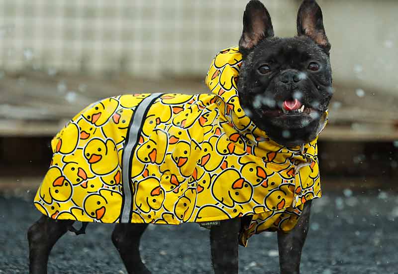
When selecting a black dog raincoat, there are several features you should prioritize. First, consider the material; a high-quality waterproof fabric is essential for effective moisture protection. Breathability is another important factor; a raincoat that allows airflow will keep your dog comfortable during walks without overheating. The fit should be snug but not restrictive, allowing for natural movements. Features like adjustable straps, reflective elements for safety, and easy-access openings for harnesses can also significantly enhance the functionality of the raincoat. By focusing on these key features, you can ensure that your black dog stays dry, comfortable, and stylish during rainy adventures.
Size and Fit Considerations
Getting the right size and fit for a black dog raincoat is crucial. To measure your dog, use a flexible measuring tape and take measurements of their neck, chest, and length from the base of the neck to the base of the tail. It's important to consult sizing charts provided by manufacturers, as sizes can vary. A well-fitted raincoat should allow your dog to move freely, so look for designs that offer a good range of motion without being too loose. Remember that a coat that’s too big can allow water to seep in, while one that's too small can restrict movement and cause discomfort. A perfect fit ensures your dog can enjoy rainy walks without feeling constricted.
Style and Design Options
The world of dog raincoats offers a plethora of style and design options that can cater to both functionality and aesthetics. From classic, simple designs to modern, trendy looks, you’ll find something that suits your black dog’s personality. Bright colors and reflective patterns are excellent choices for enhancing visibility during dim, rainy days. Some raincoats even come with hoods or additional features like pockets, which can add a touch of style while providing practical functions. Choosing a design that not only keeps your dog dry but also complements their look can make walks more enjoyable and fashionable.
Comparing Purchase Options
When it comes to purchasing a black dog raincoat, you’ll find several options available. Local pet stores, online retailers, and specialty shops all carry a range of products. It’s a good idea to compare options by reading customer reviews to gauge the quality and durability of the raincoats. Pay attention to the return policies as well; a flexible return policy allows you to exchange or return the coat if it doesn’t fit your dog as expected. Additionally, consider checking for seasonal sales or discounts, which can help you find a quality raincoat without breaking the bank. By doing thorough research, you can ensure you select the best possible option for your black dog.
Choosing the Right Raincoat for Your Black Dog
In conclusion, choosing the right raincoat for your black dog is essential for their comfort, health, and safety during rainy weather. By understanding the importance of keeping your dog dry and exploring the key features, size considerations, and style options available, you can make an informed decision that benefits both you and your furry friend. Remember to take your time comparing options and always prioritize quality and fit. With the right black dog raincoat, you can enjoy countless adventures together, rain or shine!